|
Application of
multiple regression to explaining the vote for Reagan by
state in 1984:
- The setting of the 1984
election:
- Republican President
Ronald Reagan ran against the Democratic candidate,
Walter Mondale
- How well would
Reagan do in 1984 comapred with his election in
1980?
- Walter Mondale had
won the nomination handily over Jesse Jackson, who
promised to mobilize the black vote in 1984
- What impact would
the "Jackson factor" have on turning out the
Democratic vote in 1984?
- Mondale's
running-mate for Vice President was Geraldine
Ferraro
- What impact would
the "Ferraro factor" have on turning out women to
vote for the ticket in 1984?
- Let's include all
three variables in a model to explain Reagan's vote in
1984.
- Matrix of
correlations:
- Use of Multiple
Regression in SPSS 10 to execute this
model:
- Under Analyze
in the Menu select Linear Regression
- In the "Dependent"
box, enter the name of the variable you want to
explain: Reagan84
- In the
"Independents" box enter the names of the
explanatory variables: Reagan80, PctBlack,
PctWomen
- for this analysis,
select STEPWISE [enters the variables one
at a time] in the "Method" box.
- Click on the
"Statistics" button and check
- "Estimates" for
Regression Coefficients and
- "Model Fit"
- Press
"Continue"
- Click on
"OK"
Here are the series of output boxes for the above SPSS
run:

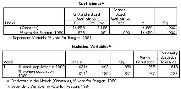
- Interpretation:
- Although three
independent variables were offered for inclusion using
the stepwise procedure, only Reagan84
was included in Model 1
- The box for the
"Excluded Variables" shows that % Black and
% Women were not significant at the .05
level and therefore were not selected for
inclusion.
Another try: Reconsidering the politics of the 1980
and 1984 elections
- In 1980, Reagan ran
against President Jimmy Carter, a southerner
- Southern states have
the highest proportions of black voters
- Perhaps Carter in
1980 ran relatively better in the south against Reagan
than Minnesotan Mondale did in 1984
- So perhaps we need to
control for the south before assessing the impact of
the Jackson factor
- Let's redo the analysis
entering the variable, South, scored 1 if the
state is one of the 11 in the deep south, or 0
otherwise.
- Here's the new
correlation matrix
- Note that the
correlation between "south" and "Reagan80" was
negative (as expected) but very small.
|
CORRELATION:
|
REAGAN80
|
PCTBLACK
|
PCTWOMEN
|
SOUTH
|
|
REAGAN84
|
0.900
|
-0.565
|
-0.513
|
0.123
|
|
REAGAN80
|
|
-0.595
|
-0.537
|
-0.082
|
|
PCTBLACK
|
|
|
0.522
|
0.511
|
|
PCTWOMEN
|
|
|
|
0.211
|
- Still, let's carry out
the new stepwise analysis using four independent
variables:
-
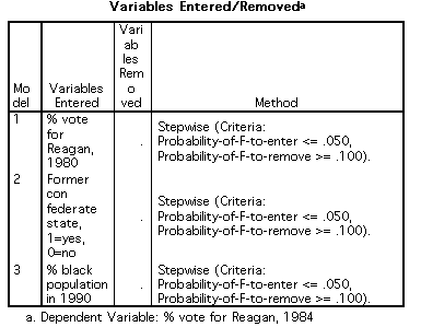
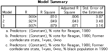 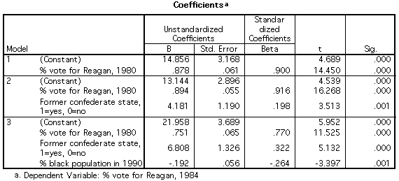 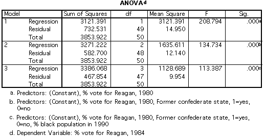 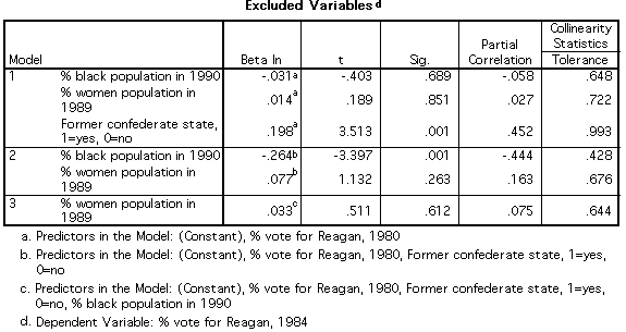
Interpreting this stepwise output
- Adding south as a
variable completely alters the analysis.
- In Model 2, South
is added to Reagan as a second explanatory
variable, raising the R2 from .81 to
.85.
- In Model 3, once
South is controlled for, %Black enters the
equation as a significant variable (.05 level), raising
the R2 to ,88.
- However, %Women
is not added into the equation to further increase the
explanation:
- As shown in the
Excluded Variables table above, it is only
significant at .612 -- which is well short of .05 and
so not added.
- In truth, there is
relatively little variance among states in % women,
making that a weak explanatory
variable.
Interpreting the regression coefficients in the
REGRESSION printout:
- REGRESSION
coefficients
- Regression
coefficients are embedded within a regression
EQUATION
- "b" coefficients
are "unstandardized" coefficients and can be
interpreted using the scale of measurement for the
raw data.
- "beta"
coefficients are "standardized" and must be
interpreted in terms of "standard deviation"
units.
- Because of the
standardization, "beta" coefficients can be
compared WITHIN equations; "b" coefficients
cannot.
- The regression
coefficients in a multiple regression equation are
"partial" coefficients because they state the
"effect" of a given independent variable on the
dependent variable while "controlling" for
effects of other variables in the
equation.
- Regression
coefficients measure CHANGE in Y, not percent
of variance explained.
-
CORRELATION coefficients:
- Measure the
STRENGTH of a relationship, i.e., the fit of
observed Y values around the line representing
predicted Y values according to a regression
equation.
- Simple
correlations pertain to bivariate relationships
involving only one independent variable and are
expressed by r.
- Multiple
correlations pertain to multivariate
relationships using multiple independent variables and
are expressed by R.
- The regression
procedure refers to the "partial" correlations of
variables not in the equation to choose which
variables (if any) are to be added to the equation
next.
- Partial
correlations computed by regression pertain
to the correlation between a dependent variable, Y,
and an independent variable, Xi, out of the
equation while "controlling for" the effects of the
other independent variables already in the
equation.
- In essence,
partial correlations express the correlation
between the residuals (i.e., deviations) of Y
regressed on Xi and the residuals around
the line of the regression equation built from the
other variables in the equation.
|

