Frequency Distributions

Use of SPSS in statistical analysis: Frequency Distributions The number of variables in the analysis determines the possible type of analysis. Univariate refers to the analysis of a single variable. Bivariate indicates analyzing the joint occurrence or covariation of two variables. Multivariate desccribes the joint covariation of more than two variables. Univariate statistics at the simplest level merely constitutes representations of distributions, which can be divided into FULL representations of raw values of observations GROUPED representations of raw values in collapsed categories SUMMARY representations of raw values of observations do not display complete information about the distribution of cases.

Full representations of distributions: raw counts of observed values

Frequency distributions: simple counts of observations pre-sorted into numerically ordered categories These can be produced with the Frequencies procedure in SPSS, which lies under the Analyze Menu.

Frequencies is suitable for nominal-scale variables: i.e., non-orderable discrete variables It is also suitable for most ordinal variables: i.e., orderable discrete variables with limited numbers of categories.   An example: FREQUENCIES for DIVISION in the states2000 data:

DIVISION SUBDIVISIONS WITHIN REGIONS Valid Cum Value Label Value Frequency Percent Percent Percent NEW ENGLAND 1 6 11.5 11.8 11.8 MIDDLE ATLANTIC 2 3 5.8 5.9 17.6 EAST NORTH CENTRAL 3 5 9.6 9.8 27.5 WEST NORTH CENTRAL 4 7 13.5 13.7 41.2 SOUTH ATLANTIC 5 9 17.3 17.6 58.8 EAST SOUTH CENTRAL 6 4 7.7 7.8 66.7 WEST SOUTH CENTRAL 7 4 7.7 7.8 74.5 MOUNTAIN 8 8 15.4 15.7 90.2 PACIFIC 9 5 9.6 9.8 100.0 . 1 1.9 Missing ------- ------- ------- Total 52 100.0 100.0 Valid cases 51 Missing cases 1

Frequencies is even suitable for interval or ratio-scaled variables IF the number categories is not great An example: bill96 (I'm using this in lieu of bush2000, but the point is the same. Strictly speaking, bill96 is a discrete, orderable variable. Practically speaking, bill96 can be considered a continuous variable--for it assumes so many values or a ratio-scaled variable--for it has intervals of know width (percentage points) and an absolute zero (0 votes) Frequencies for bill96:

BILL96 % of vote for Clinton in 1996 Valid Cum Value Label Value Frequency Percent Percent Percent 33 2 3.8 3.9 3.9 35 1 1.9 2.0 7.8 36 1 1.9 2.0 9.8 37 1 1.9 2.0 11.8 40 2 3.8 3.9 15.7 41 1 1.9 2.0 17.6 42 1 1.9 2.0 19.6 43 2 3.8 3.9 23.5 44 6 11.5 11.8 35.3 45 1 1.9 2.0 37.3 46 2 3.8 3.9 41.2 47 3 5.8 5.9 47.1 48 3 5.8 5.9 52.9 49 3 5.8 5.9 58.8 50 2 3.8 3.9 62.7 51 4 7.7 7.8 70.6 52 5 9.6 9.8 80.4 53 1 1.9 2.0 82.4 54 4 7.7 7.8 90.2 57 1 1.9 2.0 92.2 59 1 1.9 2.0 94.1 60 1 1.9 2.0 96.1 62 1 1.9 2.0 98.0 85 1 1.9 2.0 100.0 . 1 1.9 Missing ------- ------- ------- Total 52 100.0 100.0

FREQUENCIES is not useful for interval or ratio-scaled variables when the number categories is large. An example: billvote, the number of popular votes cast for Clinton in 1996, by state Because each state cast a different number of votes for Clinton, there are 51 values--one for each state

BILLVOTE Total vote for Clinton in 1996 Valid Cum Value Label Value Frequency Percent Percent Percent 66508 1 1.9 2.0 2.0 77897 1 1.9 2.0 3.9 106405 1 1.9 2.0 5.9 138400 1 1.9 2.0 7.8 139295 1 1.9 2.0 9.8 140209 1 1.9 2.0 11.8 152031 1 1.9 2.0 13.7 165545 1 1.9 2.0 15.7 167169 1 1.9 2.0 17.6 203388 1 1.9 2.0 19.6 205012 1 1.9 2.0 21.6 220197 1 1.9 2.0 23.5 220592 1 1.9 2.0 25.5 231906 1 1.9 2.0 27.5 245260 1 1.9 2.0 29.4 252215 1 1.9 2.0 31.4 311092 1 1.9 2.0 33.3 324394 1 1.9 2.0 35.3 326099 1 1.9 2.0 37.3 384399 1 1.9 2.0 39.2 385005 1 1.9 2.0 41.2 469164 1 1.9 2.0 43.1 488102 1 1.9 2.0 45.1 495878 1 1.9 2.0 47.1 612412 1 1.9 2.0 49.0 615732 1 1.9 2.0 51.0 635804 1 1.9 2.0 52.9 664503 1 1.9 2.0 54.9 670854 1 1.9 2.0 56.9 712603 1 1.9 2.0 58.8 874668 1 1.9 2.0 60.8 899645 1 1.9 2.0 62.7 905599 1 1.9 2.0 64.7 924284 1 1.9 2.0 66.7 928983 1 1.9 2.0 68.6 1024817 1 1.9 2.0 70.6 1047214 1 1.9 2.0 72.5 1070990 1 1.9 2.0 74.5 1071859 1 1.9 2.0 76.5 1096355 1 1.9 2.0 78.4 1099132 1 1.9 2.0 80.4 1567223 1 1.9 2.0 82.4 1599932 1 1.9 2.0 84.3 1941126 1 1.9 2.0 86.3 2100690 1 1.9 2.0 88.2 2206241 1 1.9 2.0 90.2 2455735 1 1.9 2.0 94.1 2533502 1 1.9 2.0 96.1 3513191 1 1.9 2.0 98.0 4639935 1 1.9 2.0 100.0 . 1 1.9 Missing ------- ------- ------- Total 52 100.0 100.0

This table has little value, for it simply says that each unique vote cast, occurs once. The key point in using Frequencies and asking for the frequency table is whether the number of categories is large, with "large" somewhat a matter of judgment.

GROUPED representations of raw values in collapsed categories

Used when the number of "raw" values is too large for easy comprehension Most typically, grouping is suitable for continuous or "quasi-continuous" variables Income Votes won in elections Population Rules for grouping continuous variables The number of intervals depends on the RANGE of the values between the low and high scores From 6 to 20 intervals usually provides for adequate variation Interval size is determined by dividing the range by number of intervals Remember that each interval is determined by its upper and lower TRUE LIMITS: The distance on the measurement scale actually enclosed by an interval when grouping data The upper true limit is half-way between the interval's apparent upper limit and the apparent lower limit of the next-higher interval Example: Ages 21-25, 26-30 ... are actually 20.6 - 25.5 and 25.6 - 30.5 Discrete variables, whether ordered or not, can be grouped usefully together when the number of original categories is large: Ethnic groups in the U.S. Nations of the world grouped into regions Grouped data are often displayed in graphs typically involve grouped data, which have distinct advantages over tables of numbers. Graphs are visually striking and thus easier to interpret and remember. Whereas numbers must be processed in digital fashion, lLnes and areas can be interpreted spatially -- in analog fashion. Good graphs are time-consuming to construct by hand, but they can be generated easily by computers. Types of graphs available under Frequencies in SPSS: HISTOGRAMS for grouped continuous data: bars should touch. BAR GRAPHS for categorical data: bars should not touch. PIE CHARTS are also for categorical data. 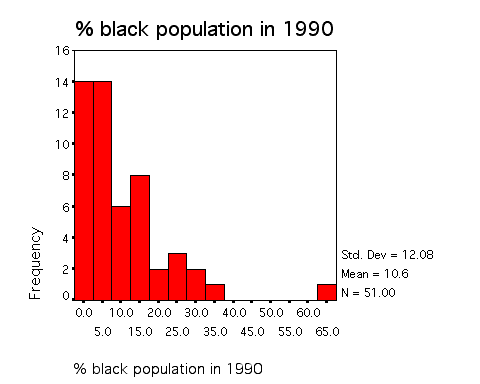First, consider HISTOGRAMS for the two variables, billvote and pctblack: By default, values are collected into several equal size intervals for plotting the histogram.

BARCHART produces a graph suitable for DISCRETE variables. Consider the example for the variable DIVISION Note the spaces between the bars. They suggest that the values are discrete, not continuous.

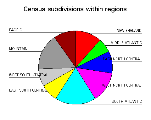
A Pie chart for the same variable is more colorful, but may be too complex for each understanding.

SUMMARY representations of raw values do not display complete information about the distribution of cases.

They provide only a single value which attempts to summarize the distribution. Because any summary throws away information, summary measures are necessarily imperfect. The two major classes of summary measures: Measures of central tendency Measures of dispersion Both of these will be taken up later this week