Linear Regression

Combining correlational analysis with linear regression Here is the simple "scattergram" that plotted how the states voted for president in 1980 and 1984. correlation, r = .90 The entries in two-dimensional space stand for the number of states that voted about the same for Reagan in each election.  The correlation in vote for Reagan between the two years is very high, meaning that one could fairly well predict a state's vote in 1984 (Y) with knowledge of the state's vote in 1980 (X)  -- IF one knew the formula for the underlying "regression line."  Determining the "regression line" that underlies the correlation coefficient:  The plot of reagan84 with reagan80 suggests that a "linear relationship" exists.  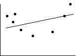One can imagine a straight line through the swarm of points. The formula for such a line is   Where: = the predicted value of the dependent variable, Yi  a = a constant, the point at which the line crosses the Y axis when X = 0 b = a coefficient representing the "slope" of the line Xi = the observed value of the independent variable for the ith case  In fact, a line can be drawn that constitutes the "best fit" in the sense that it minimizes the squared deviations of observed Ys from any alternative line.  Such a criterion for drawing a line is referred to as ordinary least squares (OLS). More formally:   Where: = sum of squared errors in prediction  The square root of these mean squared deviations is the standard error of estimate.  Computing the OLS (Ordinary Least Squares) regression line (these values are automatically computed within SPSS): The slope of the line, b, is computed by this basic formula:   In words, this is equivalent to  It is also equivalent to The formula for, a, the intercept is  Note that if there is no slope (i.e., an increase in X produces no increase in Y), b=0 Thus the second term on the right would also be 0 and the intercept, a, would be equal to the mean of the dependent variable, Y. Thus, the "slope" in the scatterplot would be a straight line from right to left, drawn at the mean of Y. Computing the regression coefficient, byx (variable Y regressed on X): Conceptually, the regression coefficient is the ratio of the covariation between both variables to the variation of the independent variable. The regression coefficient byx is an unstandardized coefficient, which means that it is calculated for the "raw" or unstandardized data. It represents the slope of the regression line--the amount of change in Y due to a change of 1 unit of X.  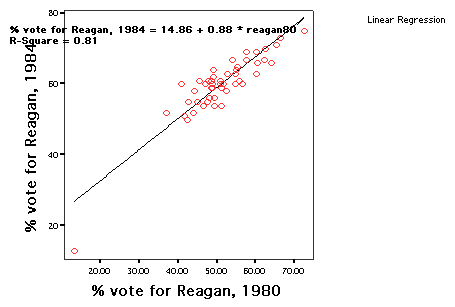Calculating b using cross-products and standard deviations: for variable Y regressed on X, Here is the line and the regression equation superimposed on the scatterplot: How to produce a scatterplot with the regression line in SPSS 10 Example: Consider the regression equation predicting to REAGAN84 from REAGAN80, as calculated by the scatterplot output: = a + b Xi  [REAGAN84 = 14.86 + (.88)REAGAN80 ] The Correlation output (from a previous run) shows   Cross-Prod Dev of REAGAN84 = 3554.4369 [Thus, SSyx = 3554] Variance of REAGAN80 = 80.95; N = 50 [Thus, SSx = 4047 (variance x N)] Calculating the regression coefficient, b:    The coefficient .88 in the regression equation means that the percentage of a state's vote for Reagan in 1984 (Yi) increased by .88 for each percentage point that the state voted for Reagan in 1980 (Xi).   If the slope is only .88, how did Reagan win more votes in 1984 than in 1980? Note the value of the intercept, which is 14.86.  Overall, Reagan ran almost 15 percentage points better in every state in 1984 than he did in 1980.  What is the relationship between b ( the slope) and r (the correlation coefficient)?    That is, if the two variables being correlated have equal standard deviations (sy = sx) Then b=r, for r would be multiplied by 1 (1/1=1) The implication of all this is the value of the slope, b, always differs from the correlation coefficient, r, to the extent that the two variables being correlated, X and Y, vary in their standard deviations, (sy and sx) Therefore, the value of b (the slope) does not necessarily indicate the value of r (the correlation). Indeed, if the two variables, X and Y, vary greatly in their standard deviations, (sy and sx), it is possible to encounter a very small slope (e.g., b=.001) and a high correlation (e.g., r=.60) Equivalent methods for calculating byx Using covariance of XY and variance of X:   Or, using r and standard deviations of the x and y variables as described in the section above,     For REAGAN84 regressed on REAGAN80:    How can we interpret the b coefficient? These coefficients refer to the slopes of the regression lines. b coefficients are interpreted as the amount of change in the dependent variable (Y) that is associated with a change in one unit of the independent variable (X). All b coefficients are unstandardized, which means that the magnitude of their values is relative to the means and standard deviations of the independent and dependent variables in the equation.  This means that the slopes can be interpreted directly in terms of the raw values of X and Y, whether the values are percents (as in the regression of REAGAN84 on REAGAN80), or dollars (as in the regression of tax paid to income earned); or mixed scales (e.g., battlefield casualties on tonnage of bombs dropped).  In the case of REAGAN84 regressed on REAGAN80, for example, b=.878 can be interpreted in terms of a state's voting percentage for Reagan in 1984 and in 1980.  Because the value of a b coefficient depends on the scaling of the raw data, which is somewhat arbitrary (should time be measured in years, months, days?), b coefficients cannot be easily compared within a regression equation.  Later, we will consider another type of regression coefficient, beta,which is standardized such that it adjusts for the different means and variances of the variables being related.  Note that there is "another" regression line for any two correlated variables, X and Y.   The product-moment correlation, r, is symmetrical-- the correlation is the same whether either X or Y is regarded as independent or dependent variables. But regression analysis is asymmetrical: when the dependent and independent variables are switched, a different formula defining the least squares line for X regressed on Y. See Schmidt, pp. 192-193, for calculating this "other" line. There is another way to measure prediction "error" in units of measurement for Y: The standard error of the estimate is the standard deviation of observed values, Y, around predicted values, Y. It is discussed in the handout from Schmidt on pp. 191-192.  The STD ERR OF EST (not computed in the scatterplot statistics) is 3.87 for REAGAN84.  The standard error of the estimate is less frequently used in statistical analysis than the coefficient of determination, r2 Comments on the effect of the pattern of plots on the regression line and the value of the correlation coefficient Regression and correlation analysis is most appropriate when the plot is linear and homoscedastic.  Linear regression analysis underestimates a curvilinear plot between variables:      A homoscedastic plot occurs when the variances of observed Y values are equal regardless of the X values. When the plot is heteroscadestic, the accuracy of predictions from X to Y depends on the value of X:  HOMOSCEDASTIC HETEROSCEDASTIC Note also that outliers -- such as Washington, D.C.--can affect the relationship--acting to either lower or raise it. Example: Go here to see the effect of dropping Washington, D.C. from the analysis. Whether one does or does not exclude a case from the analysis rests with the analyst. In this instance, the researcher might exclude Washington, D.C., which is 100% urban, because it is not really a "state."