Interpreting the Product-Moment Correlation:

Comparing measures of relationship: r and r2 r is the PEARSON PRODUCT-MOMENT CORRELATION COEFFICIENT It ranges from -1.0 to +1.0 -- indicating perfect negative and positive relationships. Thus, the SIGN of r reveals the direction of the relationship. The magnitude of r "indicates" the strength of the relationship, measured by r2 .r2 is the COEFFICIENT OF DETERMINATION It ranges from 0 to +1.0 -- indicating, respectively, the ABSENCE of a systematic relationship to a PERFECT relationship. Intermediate values have a PRE interpretation as the proportion of variance in Y that is "explained" by X -- by the regression line.   Total VariationY = Explained Variation + Unexplained Variation Total Sum of SquaresY = Explained Sum of Squares + Unexplained SS Total SSY = Regression SS + Error SS Comparing features: Like r, r2 = 0 when the variables are completely unrelated. Unlike r2, intermediate values of r do not have a PRE interpretation unless they are squared and thus transformed into r2. Thus the correlation coefficient, r, simply suggests the strength of a relationship between variables; the exact strength can be expressed only by the coefficient of determination, r2. My suspicion: researchers have tended to report r rather than r2 simply because it produced "fatter" numbers, thus making their relationships seem stronger. 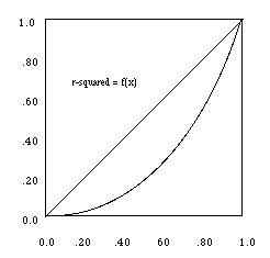The baseline represents the correlation coefficient, r, and the coordinate is r2   How about your analyses of the STATES data? Formulate a hypothesis relating political outcomes to socioeconomic characteristics. Examples and findings?   Illustration of CORRELATION output from SPSS for REAGAN84 and REAGAN80 Go to plot of the % vote for Reagan in 1984 against % vote for Reagan in 1980  Correlations % vote for Reagan, 1984 % vote for Reagan, 1980 % vote for Reagan, 1984 Pearson Correlation 1.000 0.900* Sig. (2-tailed) . .000 Sum of Squares and Cross-products 3853.922 3554.437 Covariance 77.078 71.089 N 51 51 % vote for Reagan, 1980 Pearson Correlation 0.900* 1 Sig. (2-tailed) 0 . Sum of Squares and Cross-products 3554.437 4047.562 Covariance 71.089 80.951 N 51 51 ** Correlation is significant at the 0.01 level (2-tailed).   Computing Pearson product-moment correlation from above computer printout     The values in the formula above are taken from the boldface entries in the CORRELATION output above How to produce a "scatterplot" showing the two-dimensional plot of a bivariate correlation The Graph Menu in SPSS lists the option, Scatter. . ., which produces this box, showing "Simple" as the default: Click on the "Define" button and you get this dialog box, asking you to enter variables for the Y and X axes: Click on the "OK" button, and you get this scatterplot: